Part 2: Market Power Practice Problems

Econ 502: Advanced Microeconomics

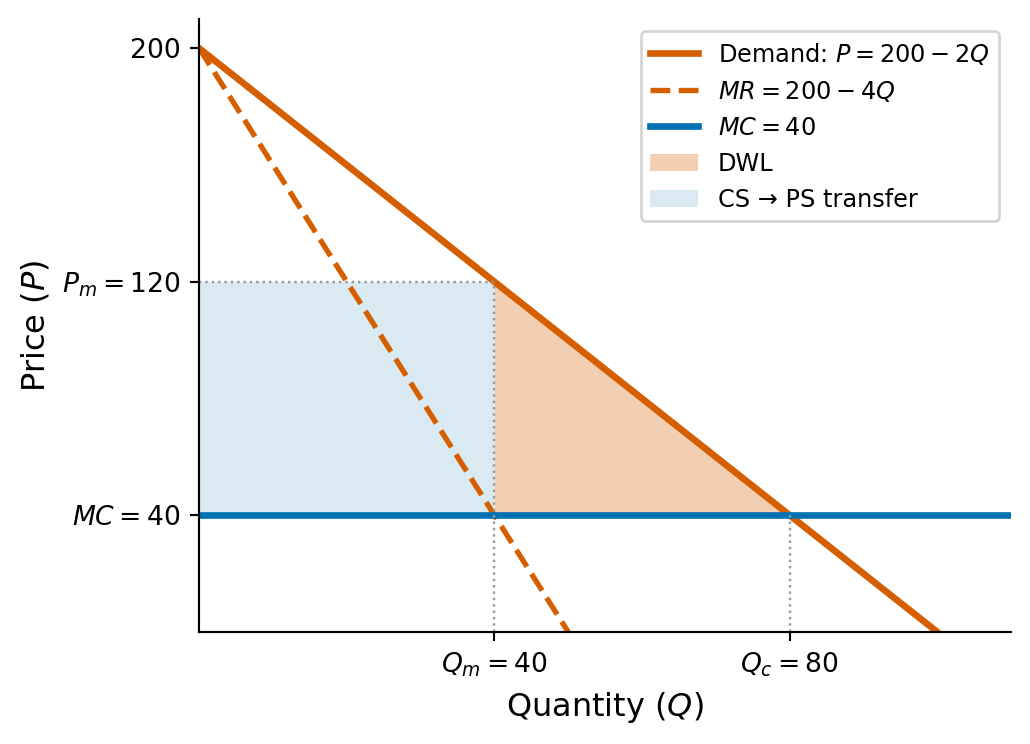
Problem 1: Monopoly Pricing

Part (a): Monopoly equilibrium

Total revenue is \(TR = P \cdot Q = (200 - 2Q)Q = 200Q - 2Q^2\). Marginal revenue:

\[MR = \frac{dTR}{dQ} = 200 - 4Q\]

Setting \(MR = MC\):

\[200 - 4Q = 40 \quad \Longrightarrow \quad Q^*_m = 40\]

\[P^*_m = 200 - 2(40) = 120\]

\[\pi = (P - MC) \cdot Q = (120 - 40)(40) = \$3{,}200\]

\[\boxed{Q^*_m = 40, \quad P^*_m = \$120, \quad \pi = \$3{,}200}\]

Part (b): Competitive equilibrium

Under perfect competition, \(P = MC\):

\[200 - 2Q = 40 \quad \Longrightarrow \quad Q_c = 80, \quad P_c = \$40\]

Consumer surplus is the area of the triangle between the demand curve and the price:

\[CS_c = \frac{1}{2}(200 - 40)(80) = \$6{,}400\]

Producer surplus is zero since the firm earns no markup (\(P = MC\) with constant marginal cost). Total surplus:

\[\boxed{TS_c = CS_c + PS_c = \$6{,}400 + 0 = \$6{,}400}\]

Part (c): Deadweight loss

Under monopoly:

\[CS_m = \frac{1}{2}(200 - 120)(40) = \frac{1}{2}(80)(40) = \$1{,}600\]

\[PS_m = (120 - 40)(40) = \$3{,}200\]

\[TS_m = 1{,}600 + 3{,}200 = \$4{,}800\]

The deadweight loss is the surplus destroyed by monopoly pricing:

\[DWL = TS_c - TS_m = 6{,}400 - 4{,}800 = \$1{,}600\]

Equivalently, the DWL is the triangle between the demand curve and MC over the range of output lost:

\[DWL = \frac{1}{2}(P_m - MC)(Q_c - Q_m) = \frac{1}{2}(80)(40) = \$1{,}600\]

\[\boxed{DWL = \$1{,}600}\]

Part (d): Lerner Index and the inverse elasticity rule

The Lerner Index measures the firm’s markup as a fraction of price:

\[L = \frac{P_m - MC}{P_m} = \frac{120 - 40}{120} = \frac{2}{3}\]

To verify using the inverse elasticity rule, we need the price elasticity of demand at the monopoly point. From the demand curve \(Q = 100 - P/2\):

\[\frac{dQ}{dP} = -\frac{1}{2}\]

\[\varepsilon_D = \frac{dQ}{dP} \cdot \frac{P}{Q} = -\frac{1}{2} \cdot \frac{120}{40} = -\frac{3}{2}\]

The inverse elasticity rule states that \(L = 1/|\varepsilon_D|\):

\[\frac{1}{|\varepsilon_D|} = \frac{1}{3/2} = \frac{2}{3} \quad \checkmark\]

\[\boxed{L = \frac{2}{3}, \quad |\varepsilon_D| = \frac{3}{2}}\]

The monopolist operates in the elastic portion of the demand curve (\(|\varepsilon_D| > 1\)), as we would expect. If demand were inelastic, the firm could increase revenue by raising the price (reducing output), so it would never be optimal to produce in the inelastic region.

Problem 2: Third-Degree Price Discrimination

Part (a): Price discrimination

The inverse demand curves are \(P_A = 100 - Q_A\) and \(P_S = 60 - Q_S\). The monopolist maximizes profit in each market separately by setting \(MR = MC\):

Adults:

\[MR_A = 100 - 2Q_A = 20 \quad \Longrightarrow \quad Q_A = 40, \quad P_A = 60\]

\[\pi_A = (60 - 20)(40) = \$1{,}600\]

Students:

\[MR_S = 60 - 2Q_S = 20 \quad \Longrightarrow \quad Q_S = 20, \quad P_S = 40\]

\[\pi_S = (40 - 20)(20) = \$400\]

\[\boxed{\text{Total profit} = 1{,}600 + 400 = \$2{,}000, \quad \text{Total output} = 60}\]

Part (b): Uniform pricing

With a single price, aggregate demand is the horizontal sum (\(P \leq 60\)):

\[Q = Q_A + Q_S = (100 - P) + (60 - P) = 160 - 2P\]

Inverting: \(P = 80 - Q/2\). Marginal revenue:

\[MR = 80 - Q = 20 \quad \Longrightarrow \quad Q = 60, \quad P = 50\]

Check that both markets are served: \(Q_A = 100 - 50 = 50 > 0\) and \(Q_S = 60 - 50 = 10 > 0\). \(\checkmark\)

\[\boxed{P = \$50, \quad Q = 60, \quad \pi = (50 - 20)(60) = \$1{,}800}\]

Note that total output is the same under both regimes (60 units). This is a general result for linear demand curves when both markets are served under uniform pricing.

Part (c): Elasticities and Lerner index

Under price discrimination, at the optimal prices:

Adults: \(\varepsilon_A = \dfrac{dQ_A}{dP_A} \cdot \dfrac{P_A}{Q_A} = (-1) \cdot \dfrac{60}{40} = -\dfrac{3}{2}\)

\[L_A = \frac{P_A - c}{P_A} = \frac{60 - 20}{60} = \frac{2}{3} = \frac{1}{|\varepsilon_A|} \quad \checkmark\]

Students: \(\varepsilon_S = \dfrac{dQ_S}{dP_S} \cdot \dfrac{P_S}{Q_S} = (-1) \cdot \dfrac{40}{20} = -2\)

\[L_S = \frac{P_S - c}{P_S} = \frac{40 - 20}{40} = \frac{1}{2} = \frac{1}{|\varepsilon_S|} \quad \checkmark\]

\[\boxed{L_A = \frac{2}{3} > L_S = \frac{1}{2}}\]

Adults get the higher markup because their demand is less elastic (\(|\varepsilon_A| = 3/2 < |\varepsilon_S| = 2\)). Adults are less price-sensitive, so the monopolist can extract more surplus from them by charging a higher price relative to marginal cost. This is the key insight of third-degree price discrimination: charge more where demand is less elastic.

Part (d): Welfare comparison

Under price discrimination:

\[CS_A = \frac{1}{2}(100 - 60)(40) = 800, \qquad CS_S = \frac{1}{2}(60 - 40)(20) = 200\]

\[\text{Total CS} = 1{,}000, \qquad \text{Profit} = 2{,}000, \qquad \text{Total welfare} = 3{,}000\]

Under uniform pricing:

\[CS_A = \frac{1}{2}(100 - 50)(50) = 1{,}250, \qquad CS_S = \frac{1}{2}(60 - 50)(10) = 50\]

\[\text{Total CS} = 1{,}300, \qquad \text{Profit} = 1{,}800, \qquad \text{Total welfare} = 3{,}100\]

\[\boxed{\text{Welfare is \$100 higher under uniform pricing}}\]

	CS	Profit	Total Welfare
Price discrimination	1,000	2,000	3,000
Uniform pricing	1,300	1,800	3,100

Price discrimination is not welfare-improving here. Consumers are worse off (\(-300\) in CS) and the firm is better off (\(+200\) in profit), but the net effect is a welfare loss of \(100\). Since total output is the same under both regimes, discrimination simply reallocates output from the more elastic market (students) to the less elastic market (adults). This reallocation is inefficient: units are moved from consumers with higher marginal valuations (students priced out at \(P_S = 40\)) to consumers with lower marginal valuations (additional adults served at \(P_A = 60\)).

Note: If the student market would be shut out entirely under uniform pricing (e.g., if \(c\) were higher), price discrimination could be welfare-improving by opening a new market.

Problem 3: Cournot Duopoly with Asymmetric Costs

Part (a): Best response functions

Firm 1 (\(MC_1 = 20\)) maximizes profit given \(q_2\):

\[\pi_1 = (120 - q_1 - q_2)q_1 - 20q_1 = (100 - q_1 - q_2)q_1\]

\[\frac{\partial \pi_1}{\partial q_1} = 100 - 2q_1 - q_2 = 0 \quad \Longrightarrow \quad \boxed{q_1^*(q_2) = 50 - \frac{q_2}{2}}\]

Firm 2 (\(MC_2 = 40\)) maximizes profit given \(q_1\):

\[\pi_2 = (120 - q_1 - q_2)q_2 - 40q_2 = (80 - q_1 - q_2)q_2\]

\[\frac{\partial \pi_2}{\partial q_2} = 80 - q_1 - 2q_2 = 0 \quad \Longrightarrow \quad \boxed{q_2^*(q_1) = 40 - \frac{q_1}{2}}\]

The best response functions are no longer symmetric: Firm 1’s intercept (50) exceeds Firm 2’s (40) because its lower MC makes any given output level more profitable. Quantities remain strategic substitutes: each firm produces less when the rival produces more.

Part (b): Nash equilibrium

Solve the two best response equations simultaneously. Substitute \(q_2^* = 40 - q_1/2\) into \(q_1^*\):

\[q_1 = 50 - \frac{1}{2}\!\left(40 - \frac{q_1}{2}\right) = 50 - 20 + \frac{q_1}{4} = 30 + \frac{q_1}{4}\]

\[\frac{3q_1}{4} = 30 \quad \Longrightarrow \quad q_1^* = 40\]

\[q_2^* = 40 - \frac{40}{2} = 20\]

\[Q^* = 60, \qquad P^* = 120 - 60 = 60\]

\[\pi_1^* = (60 - 20)(40) = \$1{,}600, \qquad \pi_2^* = (60 - 40)(20) = \$400\]

\[\boxed{q_1^* = 40,\; q_2^* = 20,\; P^* = \$60,\; \pi_1^* = \$1{,}600,\; \pi_2^* = \$400}\]

Part (c): Lerner index and market power

\[L_1 = \frac{P^* - MC_1}{P^*} = \frac{60 - 20}{60} = \frac{2}{3}, \qquad L_2 = \frac{P^* - MC_2}{P^*} = \frac{60 - 40}{60} = \frac{1}{3}\]

Firm 1 has more market power (\(L_1 = 2/3 > L_2 = 1/3\)).

To understand why, note that in Cournot equilibrium each firm’s Lerner index equals its market share divided by the market price elasticity of demand:

\[L_i = \frac{s_i}{|\varepsilon_D|}, \qquad \text{where } s_i = \frac{q_i^*}{Q^*}, \quad |\varepsilon_D| = \frac{P^*}{Q^*} = \frac{60}{60} = 1\]

\[s_1 = \frac{40}{60} = \frac{2}{3}, \quad s_2 = \frac{20}{60} = \frac{1}{3} \quad \Longrightarrow \quad L_1 = \frac{2}{3},\; L_2 = \frac{1}{3} \checkmark\]

Firm 1’s lower marginal cost lets it produce more output and capture a larger market share, which in turn gives it greater price-setting power. The Lerner index reflects market share, not cost advantage directly.

Part (d): Comparison to symmetric case (\(MC = 30\))

With \(P = 120 - Q\) and both firms at \(MC = 30\), the symmetric Cournot equilibrium gives:

\[q_i^* = 30, \quad Q^* = 60, \quad P^* = 60\]

Remarkably, total output and price are identical to the asymmetric case. This is a general result for linear Cournot models: with \(n\) firms and inverse demand \(P = a - bQ\),

\[Q^* = \frac{na - \sum_i MC_i}{(n+1)b}\]

Both cases have \(\sum MC_i = 20 + 40 = 30 + 30 = 60\), so \(Q^* = (2 \times 120 - 60)/3 = 60\) and \(P^* = 60\) in both.

Since \(P\) and \(Q\) are the same, consumer surplus is identical. The difference lies in production costs:

	\(q_1\)	\(q_2\)	Total cost	Total profit	Total welfare
Asymmetric (\(MC_1=20, MC_2=40\))	40	20	\(20(40)+40(20)=1{,}600\)	\(2{,}000\)	\(3{,}800\)
Symmetric (\(MC_1=MC_2=30\))	30	30	\(30(30)+30(30)=1{,}800\)	\(1{,}800\)	\(3{,}600\)

(Total welfare = CS + total profit = \(1{,}800 +\) total profit.)

Asymmetric costs generate higher total welfare by \(\$200\). The Cournot mechanism reallocates production from the high-cost firm (Firm 2 drops from 30 to 20 units) to the low-cost firm (Firm 1 rises from 30 to 40 units). This productive reallocation reduces total production cost for the same output, raising total surplus. In other words, when cost differences exist, even imperfect competition partially corrects the production inefficiency of a symmetric allocation.

Problem 4: Bertrand Competition

Part (a): \(p_1 = p_2 = c\) is a Nash equilibrium

We need to show that neither firm can increase its profit by unilaterally changing its price.

At \(p_1 = p_2 = c\), each firm earns zero profit (price equals marginal cost). Consider firm 1’s possible deviations:

• Raise price (\(p_1 > c\)): Firm 1 loses all customers to firm 2 (which still charges \(c\)). Firm 1’s profit remains \(\$0\). No improvement.

• Lower price (\(p_1 < c\)): Firm 1 captures the entire market but sells below cost. Firm 1’s profit is \((p_1 - c) \cdot Q(p_1) < 0\). This is strictly worse.

Since no deviation is profitable, \(p_1 = p_2 = c\) is a Nash equilibrium. \(\quad \checkmark\)

Part (b): \(p_1 = p_2 > c\) is not a Nash equilibrium

Suppose both firms charge \(p = p_1 = p_2 > c\), splitting the market equally. Each firm earns:

\[\pi = (p - c) \cdot \frac{Q(p)}{2} > 0\]

Now consider firm 1 deviating to \(p_1 = p - \epsilon\) (for small \(\epsilon > 0\)). Since the good is homogeneous and firm 1 is now cheaper, it captures the entire market:

\[\pi_1^{\text{dev}} = (p - \epsilon - c) \cdot Q(p - \epsilon)\]

For small \(\epsilon\), this is approximately \((p - c) \cdot Q(p)\), which is roughly double firm 1’s original profit. Since this is a profitable deviation, the original prices cannot be a Nash equilibrium. \(\quad \checkmark\)

Part (c): Asymmetric costs

With \(MC_1 = 10\) and \(MC_2 = 20\), firm 1 has a cost advantage.

If firm 1 sets \(p_1 = 20 - \epsilon\) (just below firm 2’s cost), it captures the entire market while firm 2 cannot profitably undercut (doing so would mean pricing below its own marginal cost).

At \(p_1 = 20\) (taking the limit as \(\epsilon \to 0\)):

\[Q = 100 - 20 = 80\]

\[\pi_1 = (20 - 10)(80) = \$800\]

Firm 2 earns \(\$0\).

\[\boxed{p_1^* = 20, \quad \pi_1 = \$800, \quad \pi_2 = \$0}\]

The low-cost firm captures the entire market by pricing at (or just below) the rival’s marginal cost. Note that if firm 1 was a monopoly, it would set \(MR = MC\), particularly: \[MR = 100 - 2Q = 10 \Longrightarrow Q = 45, \quad P = 100 - 45 = 55\]

However, in the Bertrand duopoly, firm 1 cannot charge above \(20\) without losing all customers to firm 2. Thus, the equilibrium price is determined by the rival’s cost, not by the monopolist’s optimal price.

Problem 5: Differentiated Bertrand Competition

Part (a): Best response functions

Firm 1 maximizes \(\pi_1 = (p_1 - 1)(10 - 2p_1 + p_2)\). The FOC with respect to \(p_1\) is:

\[\frac{\partial \pi_1}{\partial p_1} = (10 - 2p_1 + p_2) + (p_1 - 1)(-2) = 0\]

\[10 - 4p_1 + p_2 + 2 = 0 \quad \Longrightarrow \quad \boxed{p_1^*(p_2) = 3 + \frac{p_2}{4}}\]

By symmetry, \(p_2^*(p_1) = 3 + p_1/4\).

Prices are strategic complements: the best response is upward sloping (\(\partial p_1^*/\partial p_2 = 1/4 > 0\)). If firm 2 raises its price, firm 1’s demand rises, and it optimally charges more as well.

Part (b): Nash equilibrium

In a symmetric equilibrium \(p_1 = p_2 = p^*\):

\[p^* = 3 + \frac{p^*}{4} \quad \Longrightarrow \quad \frac{3p^*}{4} = 3 \quad \Longrightarrow \quad p^* = 4\]

\[q_i = 10 - 2(4) + 4 = 6, \qquad \pi_i = (4 - 1)(6) = \$18\]

\[\boxed{p^* = 4, \quad q_i = 6, \quad \pi_i = \$18}\]

Part (c): Why equilibrium price exceeds marginal cost

\(p^* = 4 > c = 1\), so firms earn positive profits in equilibrium. With product differentiation, a firm that slightly undercuts its rival does not capture the entire market: some customers still prefer the higher-priced firm’s product. The demand function is continuous in own price, so there is no incentive to trigger a race to the bottom. The Bertrand paradox rests on the assumption of perfectly homogeneous goods; once goods are differentiated, the “steal the whole market” logic breaks down.

Part (d): Collusion

Setting \(p_1 = p_2 = p\), joint profit is:

\[\Pi = 2(p - 1)(10 - 2p + p) = 2(p - 1)(10 - p)\]

FOC:

\[\frac{d\Pi}{dp} = 2\bigl[(10 - p) - (p - 1)\bigr] = 2(11 - 2p) = 0 \quad \Longrightarrow \quad p^{\text{col}} = 5.5\]

\[q_i^{\text{col}} = 10 - 2(5.5) + 5.5 = 4.5, \qquad \pi_i^{\text{col}} = (5.5 - 1)(4.5) = \$20.25\]

\[\boxed{p^{\text{col}} = 5.5 > p^* = 4, \quad \pi_i^{\text{col}} = \$20.25 > \pi_i^* = \$18}\]

Collusion raises prices and profits for both firms. However, the collusion point cannot be sustained as a Nash equilibrium in a one-shot game. To see why, suppose firm 2 holds the collusive price \(p_2 = 5.5\). Firm 1’s best response is: \[p_1^*(5.5) = 3 + \frac{5.5}{4} = 4.375\] Since \(4.375 < 5.5\), firm 1 has a unilateral incentive to undercut the collusive price as charging less attracts more customers and raises firm 1’s profit above \(\$20.25\). Sustaining collusion requires repeated interaction, so that the threat of future punishment (reverting to the Nash price of 4) outweighs the short-run gain from deviation.

Problem 6: Stackelberg Competition

Part (a): Cournot equilibrium

Firm 1 maximizes \(\pi_1 = (150 - q_1 - q_2 - 30)q_1 = (120 - q_1 - q_2)q_1\).

FOC: \(120 - 2q_1 - q_2 = 0 \Longrightarrow q_1^*(q_2) = 60 - q_2/2\). By symmetry, \(q_2^*(q_1) = 60 - q_1/2\).

Solving simultaneously:

\[q_i^C = 40, \quad Q^C = 80, \quad P^C = 70, \quad \pi_i^C = (70 - 30)(40) = \$1{,}600\]

\[\boxed{q_i^C = 40, \quad P^C = \$70, \quad \pi_i^C = \$1{,}600}\]

Part (b): Stackelberg equilibrium

Step 1: Follower’s best response (same as Cournot):

\[q_2^*(q_1) = 60 - \frac{q_1}{2}\]

Step 2: Leader’s problem. Firm 1 substitutes \(q_2^*\) into its profit function:

\[\pi_1 = \left(120 - q_1 - \left(60 - \frac{q_1}{2}\right)\right)q_1 = \left(60 - \frac{q_1}{2}\right)q_1\]

FOC: \(60 - q_1 = 0 \Longrightarrow q_1^S = 60\)

\[q_2^S = 60 - \frac{60}{2} = 30, \quad Q^S = 90, \quad P^S = 60\]

\[\pi_1^S = (60 - 30)(60) = \$1{,}800, \qquad \pi_2^S = (60 - 30)(30) = \$900\]

\[\boxed{q_1^S = 60,\; q_2^S = 30,\; P^S = \$60,\; \pi_1^S = \$1{,}800,\; \pi_2^S = \$900}\]

Part (c): Comparison and the top dog strategy

	Cournot	Stackelberg Leader	Stackelberg Follower
Output	40	60	30
Price	$70	$60	$60
Profit	$1,600	$1,800	$900

The leader gains from moving first (profit rises from $1,600 to $1,800), while the follower is worse off ($900 < $1,600). By committing to a large quantity before the follower acts, the leader exploits the fact that quantities are strategic substitutes: a higher \(q_1\) shifts the follower’s best response downward, inducing firm 2 to produce less. This credible commitment to “overproducing” is the “top dog” strategy: be aggressive to force the rival to back off.

Part (d): Consumer surplus and welfare

\[CS^C = \frac{1}{2}(150 - 70)(80) = \frac{1}{2}(80)(80) = \$3{,}200\]

\[TS^C = CS^C + \pi_1^C + \pi_2^C = 3{,}200 + 1{,}600 + 1{,}600 = \$6{,}400\]

\[CS^S = \frac{1}{2}(150 - 60)(90) = \frac{1}{2}(90)(90) = \$4{,}050\]

\[TS^S = CS^S + \pi_1^S + \pi_2^S = 4{,}050 + 1{,}800 + 900 = \$6{,}750\]

	Consumer Surplus	Industry Profit	Total Welfare
Cournot	$3,200	$3,200	$6,400
Stackelberg	$4,050	$2,700	$6,750

Consumers are better off under Stackelberg: higher total output drives the price down from $70 to $60, raising CS by $850. Total welfare is also higher ($6,750 vs $6,400), despite the fall in industry profit ($2,700 vs $3,200), since the consumer surplus gain more than offsets the profit loss. Stackelberg moves the market outcome closer to the competitive benchmark.