Who Can Get Away with Raising Prices?
Demand and Elasticity
ECON 201: Principles of Microeconomics
Lecture 7
Last Class: The Cost Side
\[\text{Profit} = \underbrace{P \times Q}_{\text{revenue}} - \underbrace{C(Q)}_{\text{cost}}\]
- Last class we focused on the cost side, \(C(Q)\).
- Today we focus on revenue, \(P \times Q\), which depends on the demand curve.
- Remember the trade-off: if firm set’s higher price, it will loose some consumers. How many? That depends on the demand curve.
How Much Would You Pay?
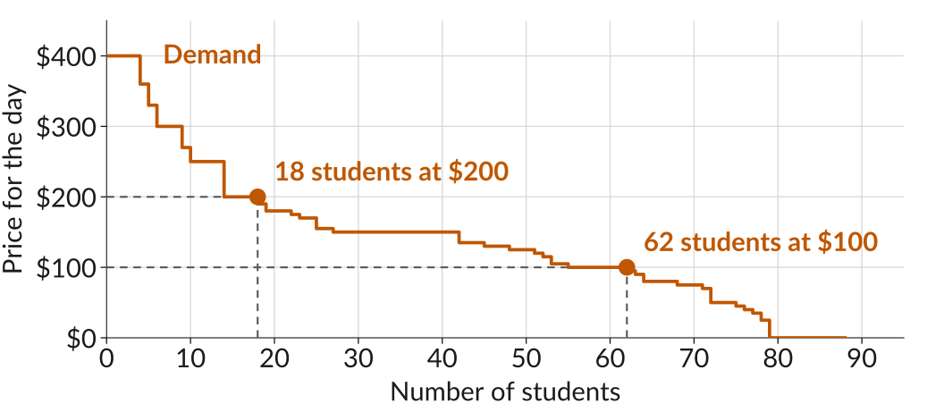
In Lecture 3, I asked for the most you would pay for a day at a Dodgers game. What you gave me was your willingness to pay (WTP), and we can use it to construct a demand curve.
Willingness to Pay
- Willingness to pay (WTP) is an indicator of how much a person values a good, measured by the maximum amount they would pay to acquire a unit of the good.
- You will go to the game if the price for the day is less than or equal to your WTP.
- At any price, demand is the number of students whose willingness to pay is at least that price.
- At $200, 18 of you have a WTP of $200 or more, so demand is 18. At $100, demand is 62.
The Demand Curve for a Dodgers Game
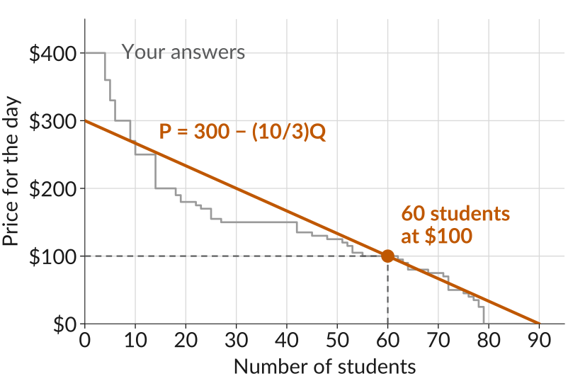
Linearizing your answers gives this demand curve:
\[P = 300 - \frac{10}{3}\,Q \quad\Rightarrow\quad Q = 90 - 0.3\,P\]
How Much Does Demand Respond?
- Sellers setting ticket prices, and economists and policymakers setting policy, often want to know how a change in price will change the quantity people buy.
- Your demand curve is \(Q = 90 - 0.3\,P\). If the price rises by $10, from $100 to $110, demand falls by 3 students.
- When \(P = 100\), \(Q = 90 - 0.3 \times 100 = 60\).
- When \(P = 110\), \(Q = 90 - 0.3 \times 110 = 57\).
- Often it is more useful to measure the change in percentage terms: if the price rises by 1%, by what percentage does the quantity fall?
- This standard measure is called the price elasticity of demand.
Price Elasticity of Demand
The price elasticity of demand is the percentage change in demand that would occur in response to a 1% increase in price:
\[\varepsilon = -\frac{\%\text{ change in demand}}{\%\text{ change in price}}\]
- Quantity falls when price increases, so the minus sign ensures that we get a positive number.
- Demand is elastic if \(\varepsilon\) is greater than 1, and inelastic if less than 1.
Elasticity of Demand for a Dodgers Game
When the price rises from $100 to $110, demand falls from 60 to 57 students.
\[\begin{aligned} \%\text{ change in price} &= \frac{110-100}{100} \times 100 = 10\% \\[0.3em] \%\text{ change in demand} &= \frac{57-60}{60} \times 100 = -5\% \end{aligned}\]
\[\varepsilon = -\frac{-5}{10} = 0.5\]
- At $100, a 1% increase in the price reduces the number of you who would go by 0.5%, so demand is inelastic.
Worksheet, Activity 1
The demand curve is given by \(Q = 90 - 0.3\,P\). Find the elasticity of demand for each $10 price rise below. At which prices is demand elastic?
\[\%\text{ change} = \frac{\text{new} - \text{old}}{\text{old}} \times 100 \qquad\qquad \varepsilon = -\frac{\%\text{ change in } Q}{\%\text{ change in } P}\]
| \(P\) rises from | \(Q\) falls from | % change in \(P\) | % change in \(Q\) | Elasticity, \(\varepsilon\) |
|---|---|---|---|---|
| $50 to $60 | ||||
| $100 to $110 | ||||
| $200 to $210 |
Four Ways to Write the Elasticity
When price changes by \(\Delta P\) and demand by \(\Delta Q\):
| Using | Elasticity | |
|---|---|---|
| 1 | Percentage changes | \(\varepsilon = -\dfrac{\%\text{ change in } Q}{\%\text{ change in } P}\) |
| 2 | Proportional changes | \(\varepsilon = -\dfrac{\Delta Q / Q}{\Delta P / P}\) |
| 3 | The fraction simplified | \(\varepsilon = -\dfrac{P}{Q} \times \dfrac{\Delta Q}{\Delta P}\) |
| 4 | The slope of the demand curve, \(\Delta P / \Delta Q\) | \(\varepsilon = -\dfrac{P}{Q} \times \dfrac{1}{\text{slope}}\) |
Worksheet, Activity 2
Use formula 3 to find the elasticity at the same three prices. Do you get the same answers as in Activity 1?
\[Q = 90 {\color{#BF5700}{\,-\,0.3}}\,P \qquad\qquad \varepsilon = -\frac{P}{Q} \times \frac{\Delta Q}{\Delta P}\]
Here, \(\Delta Q / \Delta P = -0.3\): every $1 rise in price changes demand by \(-0.3\).
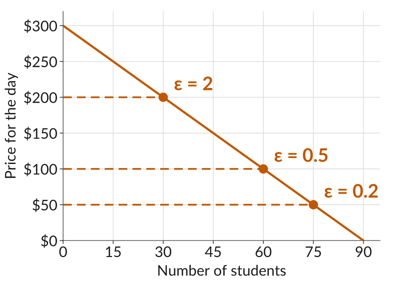
| Price, \(P\) | $50 | $100 | $200 |
| Demand, \(Q\) | 75 | 60 | 30 |
| Elasticity, \(\varepsilon\) |
Elasticity Along the Demand Curve
- As we move down a straight demand curve, the price falls and the quantity rises, so the elasticity falls.
- At a high price, few people still buy. Losing a few more is a large share of the buyers, so demand is elastic.
- At a low price, many people buy. Losing the same few is a small share of them, so demand is inelastic.
Flat and Steep Demand Curves
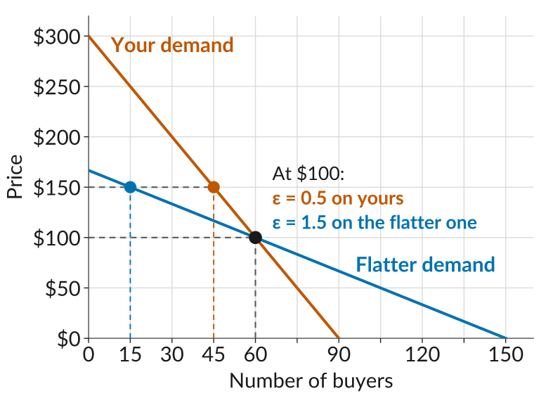
- Both curves pass through the same point: 60 buyers at $100.
- Raise the price to $150. On your curve, buyers fall to 45. On the flatter curve, they fall to 15.
- So at $100, demand is more elastic on the flatter curve: \(\varepsilon = 1.5\), against 0.5 on yours.
Why Measure How Buyers Respond?
Anyone who sets a price needs to know how buyers will respond to it.
- A firm wants to know whether a higher price brings in more revenue or less.
- A city wants to know whether a higher bus fare raises money or empties the buses.
- A government wants to know how much less people will buy of a good it taxes.
But why measure how buyers respond in percentage changes?
So we can compare goods with very different prices and units, like cars and gasoline.
Why Percentage Changes?
Suppose we want to know who responds more to price changes: people buying cars or people buying gasoline.
- A car costs tens of thousands of dollars, and gasoline costs a few dollars a gallon. A $1 price rise is nothing for a car and a big jump for gasoline.
- Car sales are counted in cars and gasoline in gallons, so “units lost for each $1 rise” cannot be compared either.
- Percentage changes remove both problems: a 10% price rise is the same size of change for a car and for a gallon of gas.
- So we compare the percentage fall in quantity for a 1% rise in price. That is the elasticity.
Why Elasticity Differs Between Goods
Demand is more elastic when buyers can easily switch or buy less:
| Reason | More elastic | Less elastic |
|---|---|---|
| Close substitutes | Coffee at Starbucks | Electricity |
| Luxury, not necessity | Concert tickets | A doctor’s visit |
| Narrowly defined market | Vanilla ice cream | Food |
| More time to adjust | Gas over five years | Gas this week |
| Big share of spending | A new car | Salt |
Elasticity in the Data: Uber
Cohen, Hahn, Hall, Levitt, and Metcalfe (2016) used Uber’s data. The app rounds the surge multiplier to one decimal.
- A surge of 1.249 shows as 1.2x, and 1.251 shows as 1.3x. Riders on each side face the same conditions, but pay 8.3% more.
- At that cutoff, ride requests are about 3% lower. What is the elasticity?
\[\varepsilon = -\frac{-3}{8.3} \approx 0.36\]
Across almost 50 million sessions, most of their estimates are between 0.4 and 0.6.
Elasticity in the Data: A Soda Tax
Seiler, Tuchman, and Yao (2021) studied Philadelphia’s 2017 tax on sweetened drinks. Prices at city stores rose by 34%.
- Sales of the taxed drinks at city stores fell by 46%, so demand there was elastic: \(\varepsilon = 46 / 34 \approx 1.35\).
- Many shoppers drove to stores outside the city. Counting those, purchases fell by only 22%, so \(\varepsilon = 22 / 34 \approx 0.65\).
- Stores outside the city are close substitutes, so demand at city stores is the more elastic of the two.
- Both numbers matter for policy: the city’s tax revenue depends on the 1.35, and how much less soda people drink depends on the 0.65.
Elasticity in the Data: Everyday Foods
Average elasticities from 160 US studies (Andreyeva, Long, and Brownell, 2010):
| Food or drink | Elasticity |
|---|---|
| Meals away from home | 0.81 |
| Soft drinks | 0.79 |
| Fruit | 0.70 |
| Milk | 0.59 |
| Eggs | 0.27 |
Every food here is inelastic. Meals out respond most, because cooking at home is a close substitute. Eggs respond least: there is no good substitute at breakfast.
Quiz 3
- Quiz 3 is Monday, September 21, and covers Lectures 5 to 7.
- Go through all the slides and work through worksheets and the practice problems before the quiz.
Sources
- Cohen, Hahn, Hall, Levitt, and Metcalfe (2016), “Using Big Data to Estimate Consumer Surplus: The Case of Uber,” NBER Working Paper 22627.
- Seiler, Tuchman, and Yao (2021), “The Impact of Soda Taxes: Pass-Through, Tax Avoidance, and Nutritional Effects,” Journal of Marketing Research 58(1).
- Andreyeva, Long, and Brownell (2010), “The Impact of Food Prices on Consumption: A Systematic Review of Research on the Price Elasticity of Demand for Food,” American Journal of Public Health 100(2).
ECON 201 · Lecture 7